Getting Started with Citibike Rebalancing

September 1, 2013

As I talked about in my previous post, I want to put together a system that will help Citibike by showing the best stations that they can rebalance. I’ve decided that I’m probably going to leave the future station prediction up to the models built over at DSSG and work on what we can do after we can predict how stations will look in 30 or 60 minutes.

Scraping in R

Parsing JSON with R is a bit silly, but I eventually came up with a decent solution that pulls in multiple fields from a decently nested JSON object without having to use either recursion or super inefficient R for loops:

require('RCurl')
require('RJSONIO')

stations.url <- getURL('http://citibikenyc.com/stations/json')

stations.json <- fromJSON(stations.url, method='C')

# put into df. note that numerics are treated as factors
stations.list <- as.data.frame(matrix(unlist(
  lapply(stations.json$stationBeanList, function(x){
    cbind(x$stationName, x$availableDocks, x$totalDocks, x$latitude, x$longitude)
    })), nrow=length(stations.json$stationBeanList), byrow=T)
  )

One minor annoyance was that I ended up with a dataframe of factors (as opposed to numerics or character vectors), so I had to go through and manually convert them into something more friendly.

Clustering mostly empty stations

I decided to try out kmeans clustering as it generally performs well. One small problem is that the algorithm requires the user to input the number of clusters. In order to examine the clusters, I used the standard practice of looking at the within groups sum of square and choosing the number of clusters where there appeared to be an “elbow” which in this case was around four (using only slightly modified code from here):

wss <- (nrow(stations.tocluster)-1)*sum(apply(stations.tocluster,2,var))
for (i in 2:15) wss[i] <- sum(kmeans(stations.tocluster,
                                     centers=i)$withinss)
plot(1:15, wss, type="b", xlab="Number of Clusters",
     ylab="Within groups sum of squares")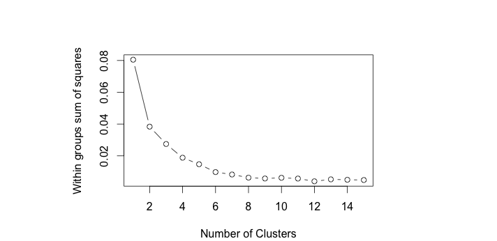

Then, we just apply the kmeans back to the input data frame, and plot the result:

stations.cluster <- data.frame(stations.tocluster, stations.kmeans$cluster)

plot(stations.cluster$long, stations.cluster$lat, pch=19,
     col = stations.cluster$stations.kmeans.cluster,
     asp = 8/6,
     xlab = "Longitude",
     ylab = "Latitude"
)

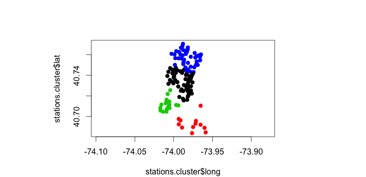
And there it is – a super basic visualization of the geographic clusters of missing bikes. The next step is to figure out how to translate those clusters into graphs (with distances as weights), and then figure out the most central point of those graphs.