Station clusters as network graphs

September 7, 2013

Picking up from the previous post, the next step of the original plan is to represent the station clusters that we built as a network graph.

Exploding each cluster

The first step here is to explode out each cluster into a data format that can be turned into a graph. I used R’s combn function to accomplish this:

graph.explode <- function(x) {
  y <- data.frame(
    t(apply(
      combn(paste(row.names(x), x[,1], x[,2], sep=","), 2), 2,
      function(i){
        i.names <- unlist(strsplit(as.character(i), split='\\,'))
        latslongs <- c(as.numeric(i.names[2]),as.numeric(i.names[3]),
                       as.numeric(i.names[5]),as.numeric(i.names[6]))
        return(c(i.names[1],i.names[4],
                 haversine.distance(latslongs[1],latslongs[2],
                                    latslongs[3],latslongs[4])))
        })))
  # cast the weight to numeric
  y[,3] <- as.numeric(as.character(y[,3]))
  # to get a better graph, we are  going to dump connections with longer
  # distances than half a mile (~.8 km)
  y <- y[y[,3] < .8,]
  return(y)
}

This function is a bit complex, so let’s map out what exactly is going on here. The function takes in a data.frame whose row names are station names and that has a column of latitudes and one of longitudes. The combn function then returns a 2 x n matrix where n is the number of combinations. I then use an apply function to calculate the Haversine distance between those two points. The haversine.distance function is given as:

degrees.to.radians<-function(degrees) {
  return(degrees*pi/180)
}

haversine <- function(long1, lat1, long2, lat2) {
  R <- 6371 # Earth mean radius [km]
  delta.long <- (long2 - long1)
  delta.lat <- (lat2 - lat1)
  a <- sin(delta.lat/2)^2 + cos(lat1) * cos(lat2) * sin(delta.long/2)^2
  c <- 2 * asin(min(1,sqrt(a)))
  d = R * c
  return(d) # Distance in km
}

haversine.distance <- function(long1, lat1, long2, lat2) {
  long1 <- degrees.to.radians(long1)
  lat1 <- degrees.to.radians(lat1)
  long2 <- degrees.to.radians(long2)
  lat2 <- degrees.to.radians(lat2)

  return(haversine(long1, lat1, long2, lat2))
}

Once I get the haversine distance between every combination of points, I simply the output to a data.frame and then transpose that it, turning the 2 x n matrix into a n x 2 data.frame. Finally, I discard point combinations that are over half a mile apart (a totally unscientific guess about how far people might be willing to walk to get a bike), and return a final data.frame. With this function, we are able to turn a set of points into data that can be represented as a network graph.

Stations as a graph

Now that we have the data in a form that can be represented as a network graph, we can go ahead and use the wonderful igraph package to plot network representation andperform calculations. Note that for the rest of the post, I am using one of the four clusters identified in the last post.

First, let’s load up the data and plot it to see what it looks like:

require('igraph')

cluster.graph <- cluster.explode(
  stations.cluster[stations.cluster$stations.kmeans.cluster==1,])

g <- graph.data.frame(cluster.graph)
l <- layout.fruchterman.reingold(g)
plot(g, layout=l, vertex.size=5, vertex.label=NA, edge.arrow.size=.1)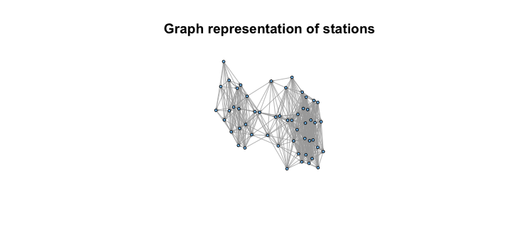

Now that we have this network representation, we can go ahead and apply some centrality measures to try and understand how to use this graph representation to make recommendations about which stations to fill first. Two centrality measures spring to mind as good use cases for this are degree centrality (measuring how many ties a node has) and possibly closeness centrality (how long it might take to traverse from some node s and other nodes). The igraph package provides the ability to calculate both of these measures, so we can take a look at the output and see how these measure stack up against how we might expect.

Degree Centrality

First up, let’s take a look at degree centrality. Degree centrality basically just measures how many edges touch a certain node. This seemingly simple method gives us a good approximation of where the most “central” nodes are located.

require('igraph')

V(g)$degcent <- centralization.degree(g)$res

deg.comps <- V(g)$degcent
deg.colbar <- cm.colors(max(deg.comps)+1)
V(g)$color <- deg.colbar[deg.comps+1]

plot(g, layout=l, vertex.size=8, vertex.label=NA, edge.arrow.size=.1,
     main='Station Degree Centrality')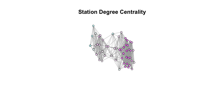

Examining this graph, we see that while the measure does a good job of finding central points in the network, it is biased towards one side of the graph, which means that taking the most centralized nodes in this measure might end up leaving parts of the city still uncovered. However, this can be worked around in the future using a function that builds a list of “close” nodes and only takes nodes that aren’t “close” to each other.

Closeness Centrality

Next up, let’s take a look at closeness centrality. Because a closeness centrality score ends up between 0 and 1, we have to do some transformations in order to see how the mesaure works graphically.

require('igraph')

V(g)$closecent <- centralization.closeness(g, mode="all")$res

cl.comps <- V(g)$closecent
cl.colbar <- cm.colors(max(round(cl.comps*100))+1)
V(g)$color <- cl.colbar[round(cl.comps*100)+1]

plot(g, layout=l, vertex.size=8, vertex.label=NA, edge.arrow.size=.1,
     main='Station Closeness Centrality')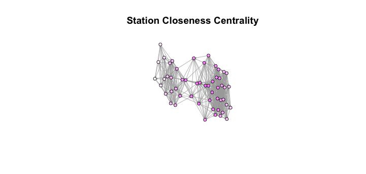

Looking at this graph, we see that the closeness meausre looks to actually lend itself towards favoring nodes that “connect” the larger parts of the graph. Because of this, it seems as though the conceptually simple degree centrality measure is the better choice going forward.

Now that we have our clusters and our centrality measure, all we have to do is parse out the data from the graph structure and nicely wrap up the results. Look for these in future posts!